FAQ
Background explanations for what you’re seeing on this site: phenotypes, polygenic scores, pleiotropy, and more.
How do I use this website?
Explore the Browse traits page to view which traits can be predicted, assess the accuracy of our predictions, and gain insight into the underlying genetic architecture of each trait.
To receive your genetic predictions, upload your genome on the VCF upload page and make sure to save your unique results code. After processing (which typically takes about an hour), you can access your trait prediction results on the Make predictions page. If there are specific traits for which you do not want to see genetic predictions, simply uncheck the box next to the trait name.
We are continually improving our prediction models and regularly adding new traits, so check back for updates!
Do you predict genetic ancestry?
Yes! We currently have a crude ancestry estimator on the Ancestry estimator page, but we will soon be upgrading it to a best‑in‑class method — stay tuned!
How should I interpret predictions?
Treat outputs as probabilistic and population-level in nature. For disease traits, we are estimating your probability (i.e. % chance) of being diagnosed with the disease by about age 75. This is not the same as lifetime risk, as you may have a 10% chance of being diagnosed with the disease by age 75, but about a 20% chance of being diagnosed with the disease by age 90.
The green and black dashed lines in the charts allow you to see how well our predicted probabilities match what actually happens. For example, when we predict that people with a given polygenic score have a certain percent x% chance of being diagnosed with the disease, we generally find that about x% of people with that polygenic score actually are diagnosed with the disease! This demonstrates that our probabilistic predictions are generally well calibrated.
- Genetic percentile: where your polygenic score sits in the population distribution.
- Predicted phenotype percentile (continuous): a rough estimate of where you may sit for that trait.
- Predicted % chance (case/control): a probability of having the disease or trait.
What is a phenotype?
A phenotype is an observable trait or outcome: a measurement (e.g., height), a lab value (e.g., LDL cholesterol), or a disease diagnosis (e.g., type 2 diabetes).
What is a polygenic score?
A polygenic score (also called a polygenic index/predictor) summarizes a person’s genetic predisposition to a trait, based on many common DNA variants—each with a small effect—that add up across the genome.
Large studies that measure both genotypes and phenotypes let us estimate these small effects. A polygenic score combines them into one number that places someone along a “genetic axis” for the trait.
What is a GWAS?
A GWAS (genome-wide association study) scans millions of genetic variants across many people and asks which variants are statistically associated with a trait.
GWAS results are the raw ingredient for building polygenic scores: they provide estimated effect sizes for each variant.
What is pleiotropy?
Pleiotropy means that some genetic variants influence more than one trait. This is often weak between unrelated traits and stronger between biologically related traits.
Genetic correlation measures how much two traits share genetic influences (from -1 to +1).
What is whole genome sequencing (WGS)?
Whole genome sequencing (WGS) reads (almost) all of your DNA and calls variants across the entire genome. “30× depth” means, roughly, each position in the genome is read about 30 times on average, which improves accuracy.
What is a Variant Call Format (VCF) file?
A VCF (Variant Call Format) file is a standard file format for storing genetic variants identified from sequencing data. It lists differences between an individual's DNA and a reference genome, including their positions, types of variants (like SNPs and indels), and genotype information. VCF files are commonly used for sharing and analyzing genetic data from whole genome or exome sequencing.
Each row in a VCF file typically represents a single variant, and the file contains both header information and data columns describing each variant’s properties. Most genetic analysis tools and services (including this one) require the VCF format for upload and processing.
How do the genetics of annual physical measurements affect my health?
Many routine physical and biomarker measurements are partly predictable from DNA. One idea is to predict biomarkers from DNA, and then plug them into a biomarker-to-late-in-life disease model.
The chart below shows how much risk of late-in-life disease changes with each standard deviation of a polygenic score. In general, it tends to be beneficial to have higher polygenic scores for biomarkers like eGFR and HDL cholesterol, and harmful to have higher polygenic scores for BMI and mean arterial pressure (blood pressure).
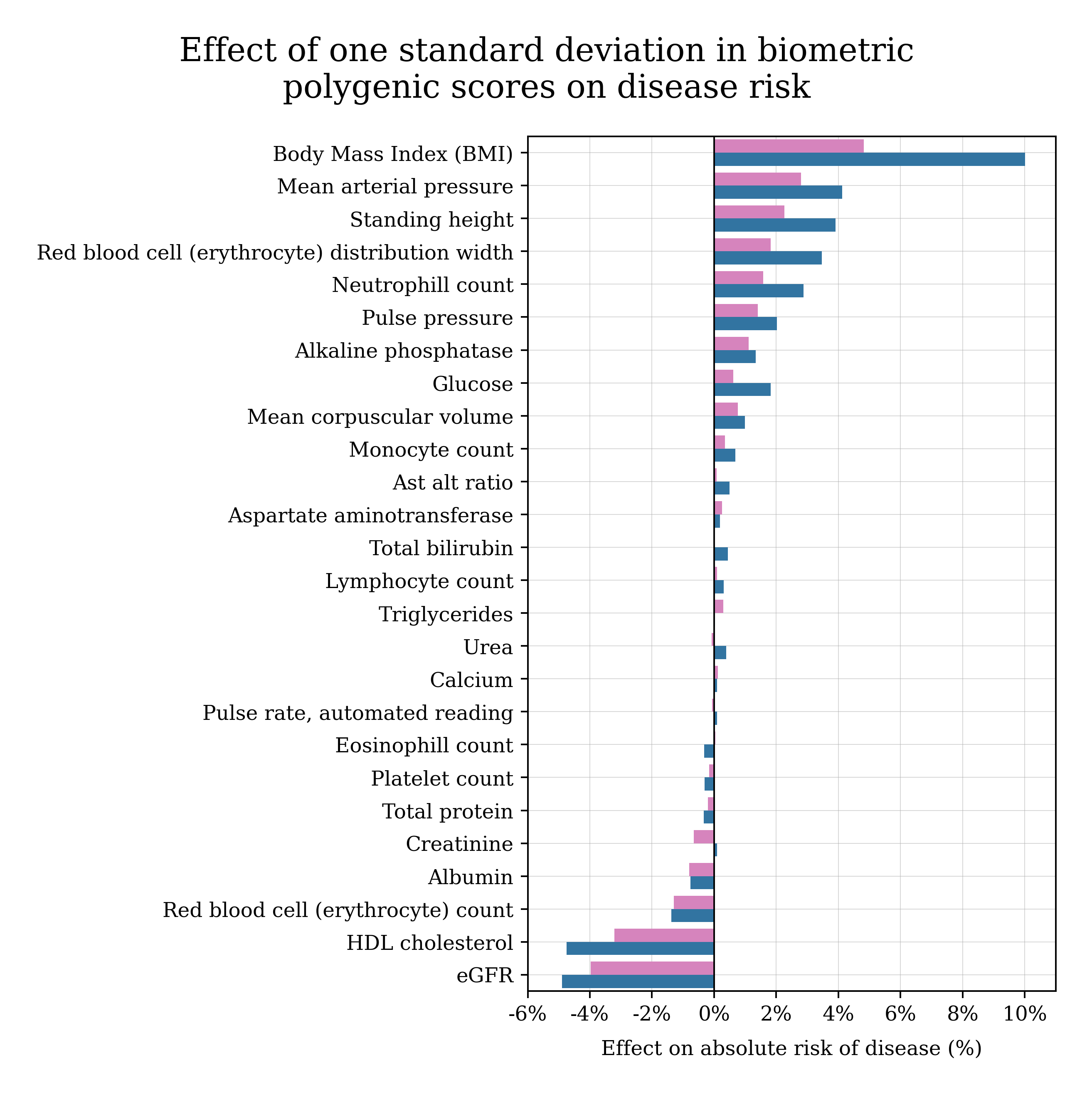
This is a population-level summary, and not a diagnosis or medical recommendation.
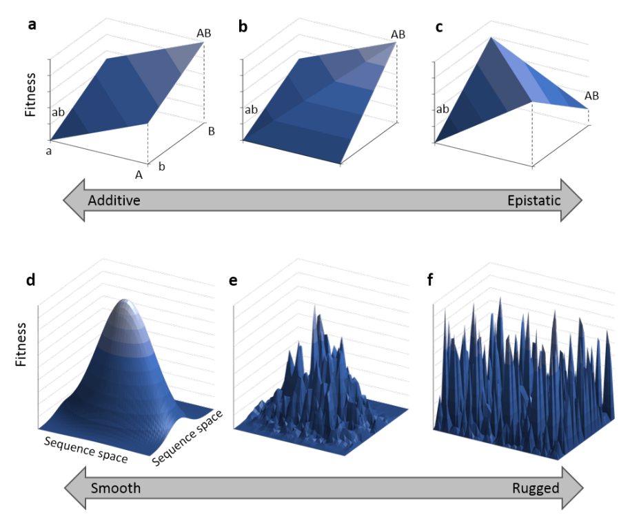
Is the genetic architecture really additive?
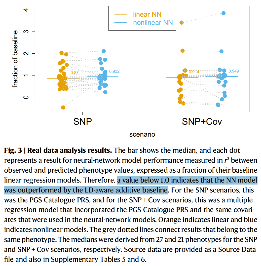
Additive models can look like a compromise, but empirically they work very well for many complex traits. Strong nonlinear genetic interactions (epistasis) are often hard to detect in practice, even when researchers try.
For example, this Nature Communications paper argues that if epistasis dominated heritability, neural networks should detect it—yet they often do not outperform additive baselines: Kelemen et al. 2025.
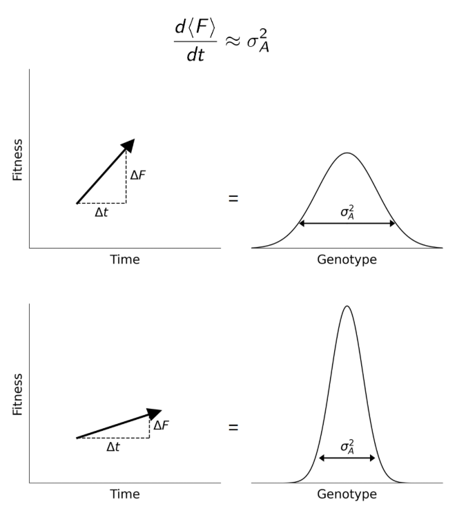
There are also evolutionary reasons to expect additive variance to matter a lot at the population level (e.g., Fisher’s fundamental theorem).
Can we predict cognitive ability from DNA?
General intelligence (“g”) captures shared variation across different cognitive tasks and predicts many life outcomes.
Current prediction is hampered by data quality and sample size. With larger cohorts and better phenotyping, prediction could improve.
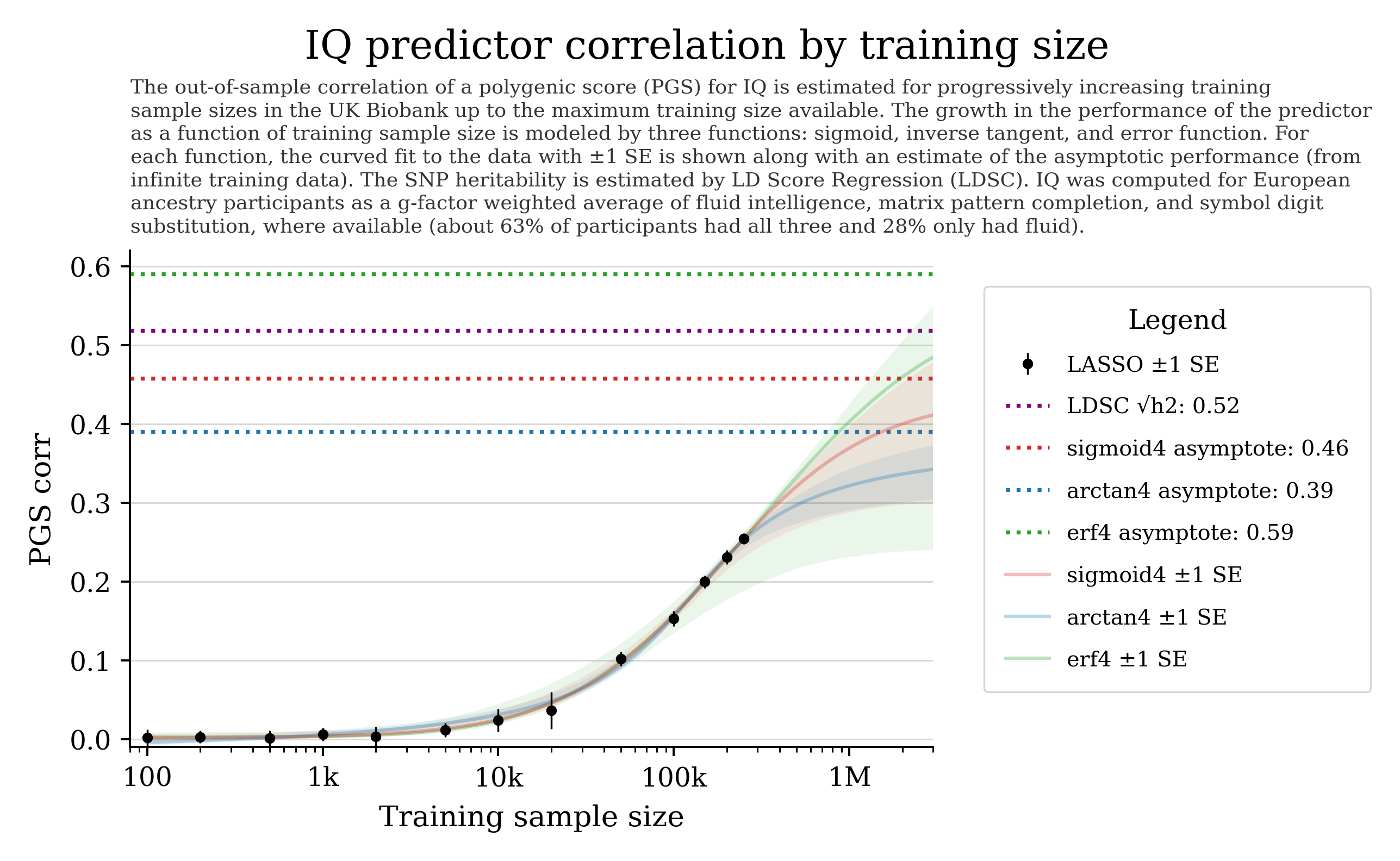
Training curves often show steady improvement with more data; some settings also show “phase transition”-like behavior.
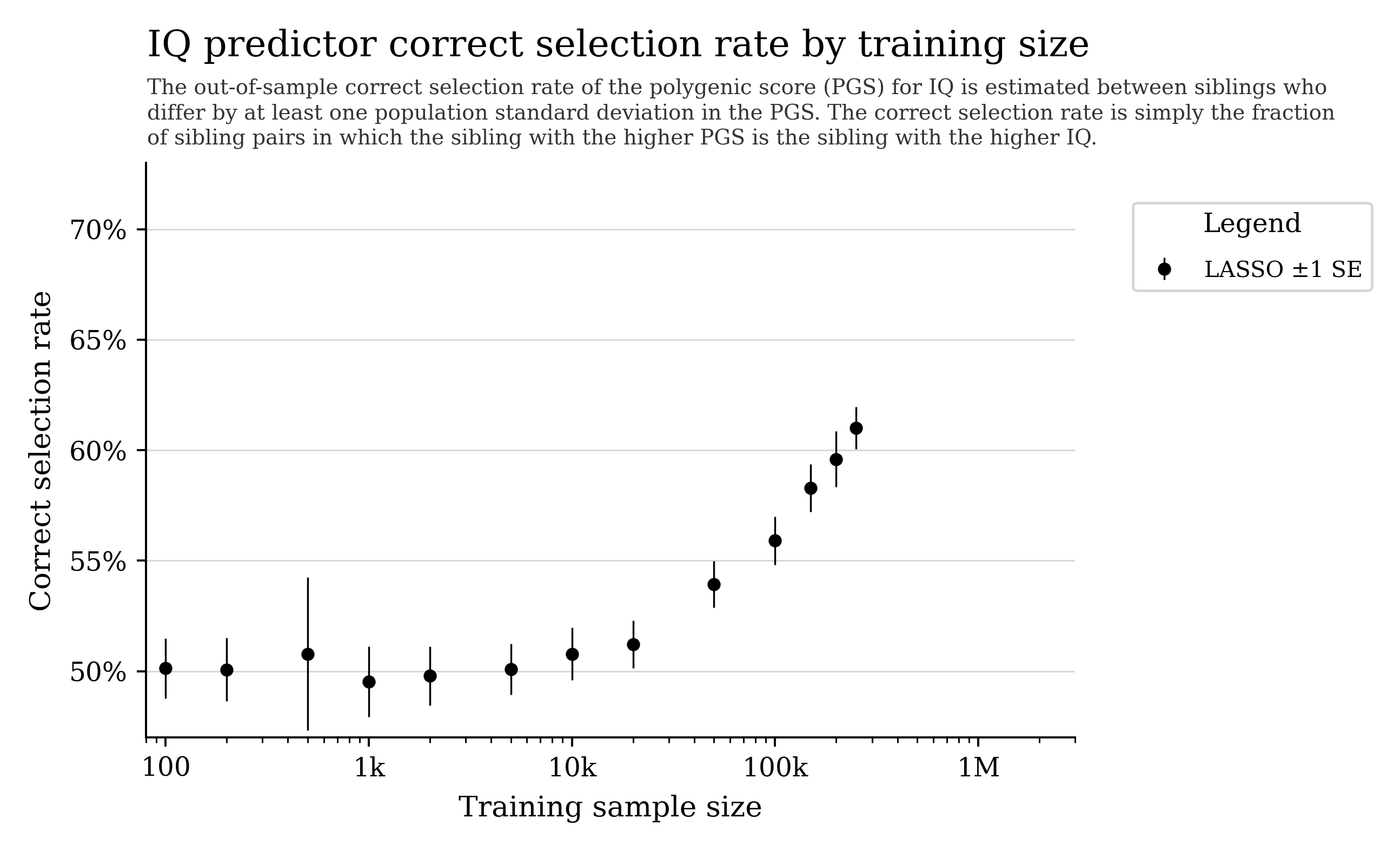
Note: some biobank cognitive tests are noisy, which can cap apparent predictability.
Privacy and data retention
Uploaded genome files are automatically deleted after 6 months. Your results code is just an identifier used to retrieve your processed outputs.